Abstract
We extend an Fst-based Bayesian hierarchical model, implemented via Markov chain Monte Carlo, for the detection of loci that might be subject to positive selection. This model divides the Fst-influencing factors into locus-specific effects, population-specific effects, and effects that are specific for the locus in combination with the population. We introduce a Bayesian auxiliary variable for each locus effect to automatically select nonneutral locus effects. As a by-product, the efficiency of the original approach is improved by using a reparameterization of the model. The statistical power of the extended algorithm is assessed with simulated data sets from a Wright–Fisher model with migration. We find that the inclusion of model selection suggests a clear improvement in discrimination as measured by the area under the receiver operating characteristic (ROC) curve. Additionally, we illustrate and discuss the quality of the newly developed method on the basis of an allozyme data set of the fruit fly Drosophila melanogaster and a sequence data set of the wild tomato Solanum chilense. For data sets with small sample sizes, high mutation rates, and/or long sequences, however, methods based on nucleotide statistics should be preferred.
LIKE many biologists, we are interested in the question of how animals and plants adapt to changes in their environment. Which regions in the genome are responsible for adaptation after climate catastrophes or the use of environmental toxins? There is growing interest in developing methods to detect loci that might be subject to selection (see Glinka et al. 2003; Ronald and Akey 2005; Vasemägi et al. 2005; Bonin et al. 2006; Li and Stephan 2006; Mealor and Hild 2006), as these loci might be functionally important (Beaumont and Balding 2004).
Individuals from different subpopulations living in different environments often vary genetically at a few key sites in their genome due to the adaptation to different local conditions. The amount of genetic differentiation can be measured from differences in allele frequencies among different populations, summarized by an estimate of the Fst-coefficient first introduced by Wright (1943). Low Fst-values may indicate balancing selection, whereas high Fst-values suggest positive directional selection.
Beaumont and Nichols (1996) developed a method, called FDIST, which starts with the calculation of θ, an estimator of the Fst-coefficient, for each locus in the sample. Then coalescent simulations are performed to generate data sets with a distribution of θ similar to the empirical distribution, from which P-values and quantiles are calculated. The quantiles of this distribution are compared with the obtained Fst-values to classify loci as selected or neutral. Simulation studies showed that this method detects at an acceptable rate loci subject to positive directional selection but lacks power to detect balancing selection (Beaumont and Balding 2004). Beaumont and Balding (2004) developed a likelihood-based approach, implemented via Markov chain Monte Carlo (MCMC), which uses a Bayesian hierarchical model similar to that of Balding (2003). In this model, each individual Fst-value for a particular population and a particular locus integrates effects that are specific to the given locus, effects that are specific to the given population, and effects that are specific to both the locus and the population (Beaumont and Balding 2004). Applications to simulated data sets with predominantly neutral loci but with some loci subject to directional or balancing selection suggested that the Bayesian method of Beaumont and Balding (2004) performed slightly better than FDIST and seemed also to detect loci subject to balancing selection. However, ideally we want to test, within a Bayesian framework, the hypothesis of whether a locus is subject to selection (Beaumont and Balding 2004). To avoid the problem of specifying appropriate alternative hypotheses we introduce an auxiliary variable for each locus effect to automatically select nonneutrally behaving locus effects. The idea to include Bayesian model selection was already considered by Beaumont and Balding (2004) but not further elaborated.
In this article, we extend the Beaumont and Balding (2004) approach. A new Bayesian auxiliary variable is introduced for each locus effect (Dellaportas et al. 2002). The new variable indicates whether a specific locus can be regarded as selected and therefore the locus effect has to be included in the model, or it can be regarded as neutral. By looking at the posterior distribution of the auxiliary variable it is possible to infer whether the locus is subject to selection. Through the prior distribution, the approach deals with the problem of multiple testing. As a prior distribution for the auxiliary variables we assume independent and identical Bernoulli distributions with parameter p, where p is a priori beta distributed. The (hyper)parameters of the beta distribution are specified in the way that only a small fraction of loci (10%) are a priori expected to be under selection. As a by-product, the efficiency of the algorithm is increased by a reparameterization, so that Gibbs sampling can be used. The method is applied to simulated data sets from a Wright–Fisher model with migration and with some loci subject to balancing or positive directional selection and to real data sets.
MATERIALS AND METHODS
Hierarchical Bayesian method:
Model:
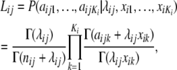
Beaumont and Balding (2004) developed a hierarchical Bayesian model, implemented via MCMC, to distinguish loci subject to selection from neutral loci. The model has two levels: a lower-level model, in which the likelihood for the allele-frequency counts is expressed as a function of Fst, and a higher-level model for the Fst-values. Allele-frequency counts at a locus within a population are modeled using the multinomial Dirichlet likelihood. This likelihood arises in a simple migration–drift model; for derivations see Balding and Nichols (1995) and Balding (2003). The multinomial-Dirichlet likelihood can be conveniently expressed in the form
 |
(1) |
where aijk, with i = 1, … , I (I is the number of loci), j = 1, … , J (J is the number of populations), and k = 1, … , Ki (Ki is the number of alleles at locus i), denotes the count of allele k in population j at locus i,  denotes the sample size, and xik is the frequency of allele k at locus i in the migrant gene pool. The scaling parameter λij is defined as
 |
As the allele-frequency counts corresponding to distinct loci and different subpopulations are assumed to be mutually independent, the joint likelihood is given by
 |
The precision of the estimates is improved when information about  is shared across loci and subpopulations by employing a hierarchical model. Each
  can be seen as a combination of contributions from locus-specific effects, such as mutations and some forms of selection, and population-specific effects, such as effective population size, migration rates, and population-specific mating patterns. These effects are included using a regression approach. Beaumont and Balding (2004) chose the logistic regression model
 |
or equivalently
 |
where αi is a locus effect, βj a population effect, and γij an interaction term representing a specific locus-by-population effect. The average Fst-value for a particular locus i is obtained by using its locus effect, the average over the population effects, and the average of the corresponding interaction effects with each population (M. A. Beaumont, personal communication). Gaussian priors f, as defined in Beaumont and Balding (2004), are used for the regression parameters αi, βj, and γij. The means and variances were selected in the way that the implied prior distribution for each  has nonnegligible density over almost the whole interval from zero to one. For
  , a (multivariate) uniform distribution is chosen as a prior distribution.
Further method development:
For determining loci that might be subject to selection, the primary interest is directed toward the posterior distribution of the locus effects. A high positive value of αi suggests that locus i might be subject to positive directional selection, whereas a negative value indicates balancing selection. Ideally, we want to assign a posterior probability to each hypothesis of the form αi = 0. In this way, the posterior probability indicates whether a locus i is neutral and hence has a zero locus effect or is subject to selection. To avoid the specification of alternative hypotheses, we use a reparameterization and introduce an additional Bernoulli-distributed auxiliary variable δi to indicate whether locus i might be subject to selection (Holmes and Held 2006). This approach also deals with the problem of multiple testing of many genomic locations, as the number of tested loci is taken into account through the prior distribution of the auxiliary variables.
Reparameterization:
The original framework used the variables αi, βj, γij, and  . Now, a new variable ηij is introduced,
 |
(2) |
which creates a new layer in the definition of  , as now the
  -value only depends on ηij directly, and ηij depends on αi and βj. The γij values are no longer sampled but the ηij values are. Of course, the γij values can be recalculated on the basis of ηij, αi, and βj. The implied prior distribution of ηij | αi, βj is given by
 |
where μγ is the prior mean of γ and  is the prior variance of γ. The prior distributions for αi and βj remain unchanged.
Introduction of Gibbs variable selection:
To indicate whether locus i might be neutral, or subject to selection, Gibbs variable selection was applied (for a recent review see Dellaportas et al. 2002). In this method, additional 0–1 random variables δi with i = 1, … , I were included in the model specification, so that
 |
The indicator vector δ shows which of the I possible locus effects are present in the model and, therefore, are assumed to be nonneutral. From the posterior distribution of the δi it is possible to infer whether a locus is subject to selection. The prior distribution of ηij changes to
 |
It would be also possible to exclude the corresponding locus-by-population effect if a locus is considered as neutral. However, we decided to keep this interaction term as it might indicate a selective pressure that is present just for a specific population at this locus.
As a prior distribution for δi with i = 1, … , I, we assume  independently and
  . We selected the hyperparameters of the beta distribution to achieve a nonnegligible density over the whole interval from zero to one and a biologically realistic prior expectation of the number of loci subject to selection. Using the law of iterated expectations, it follows that
 |
The prior distribution for the locus effects changes to αi ∼ N(0, 10), as
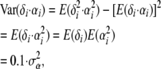 |
so that the variance of 1 is ensured, as used in Beaumont and Balding (2004).
Implementation:
The goal is to obtain values from the posterior distribution (proportional to the product of the likelihood and the prior distributions), which, for the original algorithm, takes the form
 |
(Here, the prior distributions for α, β, γ, and x are independent.) This is achieved by MCMC on the basis of iteratively updating the corresponding conditional distributions (full conditionals) (Besag et al. 1995). The estimation procedure is implemented as a Metropolis–Hastings Monte Carlo algorithm. At each step, the algorithm proposes a Gaussian update for each αi, each βj, and each γij, using the corresponding current parameter value as the mean. The variances can be chosen arbitrarily, but the choice can be optimized for achieving fast convergence. Ideally, the variances should be adapted to achieve acceptance rates between 25 and 45% (Gelman et al. 1996). Here, the variance for αi is initialized with 1.22, the variance for βj with 0.62, and the variance for γij with 1.42. If the acceptance rates are not within the desired interval after the burn-in iterations, the variances are adapted by the addition or the subtraction of 0.1 (if the variances are <0.1 only 0.01 is subtracted) and the chain is restarted. Since the normal distribution is symmetric around the mean, the update is accepted or rejected as in the Metropolis algorithm. The frequencies  are also updated, one locus at a time. The proposed value is chosen from a Dirichlet distribution with the mean proportional to the current values
 |
where the ci are locus-dependent constants used to adapt the acceptance rates. To initialize the constants ci dependent on Ki a simple regression function is used. In the case that the acceptance rates are not between 25 and 45% after the burn-in iterations, the constants ci are increased or decreased by 2% for every percentage of deviation from a target acceptance rate of 35% and the burn-in interval is repeated. When using a Dirichlet distribution as a proposal distribution the frequencies xik can become very small. To avoid this, a minimum allele frequency of 10−3 is used. Since the Dirichlet distribution is not symmetric, a Metropolis–Hastings update is required for  (Beaumont and Balding 2004).
As a consequence of introducing ηij, the full conditional distributions of αi and βj are normal distributions, so that it is now possible to sample directly from them, since
 |
where
 |
Hence
 |
with
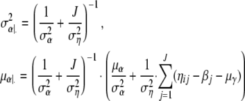 |
For the derivation of  and μα|· see, e.g., Bernardo and Smith (1994, p. 439). Analogously, we have βj ∼ N(μβ|·,
  ) with
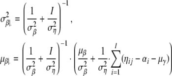 |
For the ηij the full conditional distribution
 |
is obtained, with Lij defined as a multinomial Dirichlet likelihood as in Equation 1. For updating the ηij a random-walk proposal
 |
is used, where  is initialized with 1.42 and adapted as described above for αi, βj, and γij to reach acceptance rates between 25 and 45%. The update is accepted as in the Metropolis algorithm.
One of the main advantages of this reparameterization is that the simulation can be performed more efficiently, as it is now possible to sample directly from the full conditional distributions. This method is also known as Gibbs sampling (Gilks et al. 1996). One potential problem might be that the posterior correlation between ηij and αi, βj (see Equation 2) might cause slow mixing and, therefore, slow convergence (Holmes and Held 2006). To illustrate the relative efficiency change of the reparameterization over the original method, the total CPU run time was recorded for both methods and the “effective sample size” (ESS) calculated. ESS is an estimate of the number of independent samples that would be required to obtain a parameter estimate with the same precision as the MCMC estimate based on N dependent samples (here N = 10,000). ESS can be interpreted as a measure of the information content of the MCMC samples. An ESS value close to N indicates that the MCMC samples are virtually uncorrelated. The effective sample size is calculated as the number of MCMC samples drawn divided by the autocorrelation time τ, which is defined as
 |
(3) |
where ρ(s) is the autocorrelation at lag s and measures the degree of association between sampled values of the monitored Markov chain separated by lag s. As the real autocorrelations are estimated by the sample autocorrelations, it is necessary to cut off the estimation of τ at an s-value v where the autocorrelations are sufficiently close to zero. The inclusion of estimates for much higher lags would add too much noise (Kass et al. 1998). The cutoff value v is determined using the initial monotone sequence estimator (IMSE) by Geyer (1992). Define
 |
and let r be the largest integer such that Φ(s) > 0 and Φ(s) is monotone for s = 1, … , r; then v is defined as v = 2 · r + 1 (Geyer 1992).
Introducing the auxiliary variable δi, the updates of βj and ηij are unchanged but αi is substituted by δi · αi. If δi = 1 the update of αi also stays unchanged. In contrast, αi is sampled from its prior distribution if δi = 0. Each element δi is thereby updated as part of the algorithm. The full conditional distribution of δi is given by
 |
whereby the parameter p is updated every iteration by sampling from its full conditional distribution
 |
Interpretation:
In the original setting by Beaumont and Balding (2004), a posterior distribution for αi is classified as significantly positive and therefore subject to positive directional selection if its 5% quantile is positive or equivalently if P(αi < 0 | data) ≤ 0.05. It is classified as significantly negative and therefore subject to balancing selection if its 95% quantile is negative or equivalently if P(αi < 0 | data) ≥ 0.95. In the following, the posterior probability P(αi < 0 | data) is also referred to as a Bayesian P-value.
Using Gibbs variable selection the posterior probabilities P(δi = 1 | data) instead of the Bayesian P-values are used to detect significant loci. In this way, a locus i is classified as being subject to selection if P(δi = 1 | data) is greater than some cutoff value that will be set by means of the simulation study results. To classify a nonneutral locus subject to positive directional or balancing selection we use the Fst-value at the smallest observed posterior probability P(δi = 1 | data) as a threshold. Selected loci with a smaller Fst-value are classified as subject to balancing selection, and those that have a larger Fst-value are classified as subject to positive directional selection.
In the context of selection, the locus-by-population effects γij might also be important. For example, a large positive value of γij might indicate a population in which local positive selection has driven an allele to fixation whereas this selection pressure can be weak or absent for that locus in the other populations. As the full conditional distribution of γij does not combine information across loci or populations, only extremely large selective influences can be found by inspecting the γij values (Beaumont and Balding 2004).
Simulation study:
To compare the behavior of the different methods and to assess their performance in detecting nonneutrally behaving loci we simulated gene-frequency data from a Wright–Fisher model with migration, which is similar to that of Beaumont and Balding (2004). In our simulations, all populations are assumed to have the same size, N = 10,000 chromosomes. Chromosomes in the current generation are replaced with immigrants. The immigration rate is defined by  , whereby the value of F is either set to a fixed value (e.g., 0.2) or sampled from a beta distribution, with parameters 0.25 and 2.25 as given in Beaumont and Balding (2004), to allow variable immigration rates over the populations. Then the next generation is sampled according to a specified selection coefficient s. The algorithm is repeated for T generations. In all analyses, we used 1000 generations, which should not lead to any equilibrium, but should reflect the selection coefficient. A selective sweep is assumed to take ∼
 generations. Assuming the advantage of a selected allele to be s/2, which is described in more detail in appendix a, the choice of T should be sufficiently large for a selection coefficient of 0.1. For selection coefficients that are ≪0.1 we expect the results to be worse. To allow for adaptive selection the attributes “neutral,” “red,” or “blue” are assigned at random and independently to the populations. The consequence is that the number of populations for which a selective pressure exists at a locus under selection is random. In neutral populations all alleles have the same fitness. After 1000 generations, a specified number of chromosomes is sampled with replacement to represent the allele frequencies for the given locus and population. The model is repeated for all populations and all loci to get a complete simulated data set, where we used within a data set the same selection coefficient for loci subject to balancing and positive directional selection. A detailed description of the simulation study design is given in appendix a.
We generated eight data sets, each of which consists of 1000 loci and 10 populations per locus to systematically test the power of the different methods. Focus was set on the influence of different selection coefficients but also on the influence of sample size and migration rate. The details and properties of the different data sets are given in Table 1.
TABLE 1.
Parameter values of the data sets simulated from the Wright–Fisher model with migration
| Identifier | Selection coefficient s | Sample size | No. of populations per locus | No. of neutral loci | No. of direct- selection loci | No. of balancing- selection loci |
|---|---|---|---|---|---|---|
| s100 | 0.1 | 100 | 10 | 900 | 50 | 50 |
| s050 | 0.05 | 100 | 10 | 900 | 50 | 50 |
| s020 | 0.02 | 100 | 10 | 900 | 50 | 50 |
| s100-Fb | 0.1 | 100 | 10 | 900 | 50 | 50 |
| s050-Fb | 0.05 | 100 | 10 | 900 | 50 | 50 |
| s020-Fb | 0.02 | 100 | 10 | 900 | 50 | 50 |
| s100-Fb-40 | 0.1 | 40 | 10 | 900 | 50 | 50 |
| Neutral | 0.0 | 100 | 10 | 1000 | 0 | 0 |
The addition of “Fb” to the identifier indicates that F ∼ Be(0.25, 2.25) instead of F = 0.2 leading to variable immigration rates.
Real data sets:
As in Beaumont and Balding (2004), the Drosophila melanogaster allozyme data set of Singh and Rhomberg (1987) was analyzed. The allele-frequency table for this data set is provided with the program FDIST 2 (http://www.rubic.rdg.ac.uk/∼mab/software/fdist2.zip) and includes allele counts for 61 polymorphic loci in 15 geographically distant populations of D. melanogaster. The considered populations as given in the allele-frequency table are as follows: Ottawa, Canada (OTT) (80 iso-female lines); Hamilton, Ontario, Canada (HAM) (161); Amherst, Massachusetts (MAS) (121); Brownsville, Texas (TEX) (121); La Plata, Argentina (ARG) (38); Sweden (SWE) (40); Ukraine (UKR) (44); Central Asia (CAS) (40); France (FRA) (81); Benin, West Africa (WAF) (114); Central Africa (CAF) (68); Seoul, Korea (KOR) (132); Taiwan (TAI) (80); Ho-Chi-Minh City, Vietnam (VIE) (80); and Fairfield, Australia (AUS) (100). The loci are mostly di- or triallelic. The maximum number of alleles for a locus is nine (Singh and Rhomberg 1987).
The second data set was published by Arunyawat et al. (2007) and contains sequences of the wild tomato species Solanum chilense distributed from northern Chile to southern Peru. The data set includes four different populations: Antofagasta, Chile; Tacna, Peru; Moquegua, Peru; and Quicacha, Peru. For this data set, eight loci were examined: CT066, CT093, CT166, CT179, CT198, CT208, CT251, and CT268. There were five to seven (diploid) individuals for each population, leading to 2 sequences from each individual for each locus. Therefore, the sample size is 10–14 sequences. The total length of individual loci (including indels) ranges from 778 to 1887 bp. An allele-frequency table was calculated treating each distinct haplotype at a locus as a new allele. The numbers of haplotypes for the loci vary between 23 and 30.
Environment details:
All analyses were run on an Intel Core 2 Duo T7200 processor with 1024 MB DDR-2-RAM under Kubuntu 7.04 (Feisty Fawn). Each algorithm was run to obtain 10,000 output samples for each variable. In the case of the real data sets the algorithm was run for 1,000,000 post burn-in iterations using a thinning interval of k = 100. For the 1000-locus simulations we used 250,000 post burn-in iterations and a thinning interval of k = 25. To check convergence standard diagnostic tests were applied. The analysis of the 1000-locus simulation described in Table 1 took ∼9 hr.
The executable C-files of the different algorithms used in this study are available on request from A. Riebler. Additional R programs to visualize and analyze the results as well as the data sets used in this study are also available. All programs were developed under SuSE Linux 10.0 and Kubuntu 7.04 (Feisty Fawn).
RESULTS
Simulation study results:
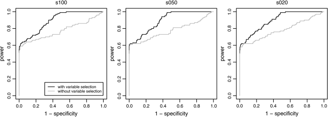
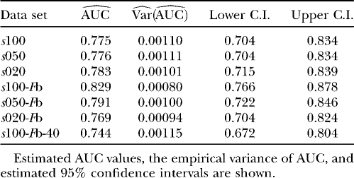
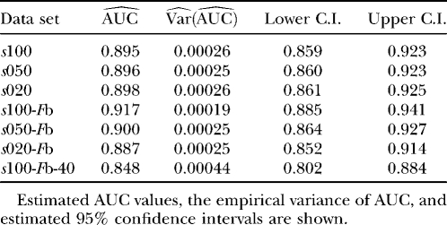
We used simulation studies to discuss the quality of the different methods in detecting loci subject to selection and to determine a suitable cutoff value for the reparameterized method with variable selection. For these purposes seven simulated data sets with predominantly neutral loci but with some loci subject to balancing or positive directional selection and one neutral data set were generated (see Table 1). The reparameterized method without variable selection is expected to increase the efficiency of the original method by Beaumont and Balding (2004), which will be confirmed by the application to the D. melanogaster data of Singh and Rhomberg (1987). Since this method is only a reformulation, the original method is not used in this simulation study. The power of the methods was assessed by a receiver operating characteristic (ROC) analysis. For detailed descriptions, compare appendix b. We generated ROC curves for all seven (nonneutral) simulated data sets. A ROC curve is a graphical plot of the power vs. (1 − specificity) for a binary classification system whereby the cutoff value is varied. In this analysis we did not distinguish between loci subject to balancing and directional selection. For all simulations we got very similar ROC plots, three of which are shown in Figure 1. It is obvious that the ROC curve of the method with variable selection is nearly always above the ROC curve of the method without Bayesian variable selection. We also tried a uniform prior distribution for the probability of including a locus effect that resulted in similar ROC curves. To measure the quality of the different methods the area under the ROC curve (AUC) was used. A perfect ROC curve has the value AUC = 1.0. In contrast, an uninformative test has AUC = 0.5 (Pepe 2003). The AUC values and the corresponding 95% confidence intervals are shown in Table 2 for the method without Bayesian variable selection and in Table 3 for the method with Bayesian variable selection. Since the scale for the AUC is restricted to (0, 1), the confidence intervals were calculated on the logit scale (Pepe 2003). To compare the empirical ROC curves we used the difference in estimated AUC values (see appendix b). The null hypothesis that the AUC value of the method with variable selection is not higher than the AUC value of the method without variable selection is tested by comparing the value of  with the 99% quantile (2.326) of a standard normal distribution (Pepe 2003). The obtained test statistics are shown in Table 4. In all cases the values of the test statistic are much larger, so the null hypothesis was rejected. This means the AUC was significantly higher for the new Bayesian variable approach.
Figure 1.—
ROC curves of three simulated data sets analyzed with the reparameterized method without Bayesian variable selection and with Bayesian variable selection. The power, also known as the true positive rate, is plotted against the false positive rate. Similar ROC curves are obtained for the other simulated data sets.
TABLE 2.
ROC analysis of the simulation results for the method without Bayesian variable selection
TABLE 3.
ROC analysis of the simulation results for the method with Bayesian variable selection
TABLE 4.
Comparison of the empirical ROC curves
The predictions are reasonably well calibrated; for example, predictions with 10% probability occur ∼7–8% of the time with a lower 95%-confidence limit between 5 and 6% and an upper 95%-confidence limit between 9 and 11%. Predictions with 5% probability occur ∼5–6% of the time with a lower 95%-confidence limit between 3 and 4% and an upper 95%-confidence limit between 6 and 7%.
By means of the results of the simulation studies we determined a threshold value for the reparameterized method with variable selection of 0.17 for classifying a locus as being subject to selection. We decided thereby to control the false positive rate and used the threshold value that achieved a specificity of at least 98% in all simulated data sets. A priori the probability for a value >0.17 is 20%. The results of the application to the simulated data sets are shown in Table 5. In comparison the results for the method without Bayesian variable selection, which uses the classification criterion described in the previous section, are shown in Table 6.
TABLE 5.
Simulation results for the method with Bayesian variable selection
| True: | Balancing selection
|
Neutrality
|
Directional selection
|
|||||||||
|---|---|---|---|---|---|---|---|---|---|---|---|---|
| Classified: | Balancing | Neutrality | Directional | Balancing | Neutrality | Directional | Balancing | Neutrality | Directional | Specificity | Power | |
| s100 | 9 | 41 | 0 | 8 | 890 | 2 | 0 | 0 | 50 | 0.99 | 0.59 | |
| s050 | 12 | 38 | 0 | 7 | 889 | 4 | 0 | 0 | 50 | 0.99 | 0.62 | |
| s020 | 7 | 42 | 1 | 5 | 893 | 2 | 0 | 0 | 50 | 0.99 | 0.57 | |
| s100-Fb | 13 | 37 | 0 | 8 | 889 | 3 | 0 | 0 | 50 | 0.99 | 0.63 | |
| s050-Fb | 10 | 39 | 1 | 5 | 894 | 1 | 0 | 0 | 50 | 0.99 | 0.60 | |
| s020-Fb | 3 | 47 | 0 | 8 | 888 | 4 | 0 | 0 | 50 | 0.99 | 0.53 | |
| s100-Fb-40 | 6 | 43 | 1 | 15 | 883 | 2 | 0 | 0 | 50 | 0.98 | 0.56 | |
| Neutral | 1 | 999 | 0 | 1.00 | ||||||||
Numbers of loci simulated under balancing selection, neutrality, and directional selection that were classified in each category by the reparameterized Bayesian regression analysis including variable selection are shown. A locus was classified as subject to selection if P(δi = 1 | data) ≥ 0.17 and otherwise was classified as neutral. For nonneutral loci the corresponding Fst-value was used to decide whether the locus is subject to directional or balancing selection.
TABLE 6.
Simulation results for the method without Bayesian variable selection
| True: | Balancing selection
|
Neutrality
|
Directional selection
|
|||||||||
|---|---|---|---|---|---|---|---|---|---|---|---|---|
| Classified: | Balancing | Neutrality | Directional | Balancing | Neutrality | Directional | Balancing | Neutrality | Directional | Specificity | Power | |
| s100 | 10 | 38 | 2 | 57 | 840 | 3 | 0 | 0 | 50 | 0.93 | 0.60 | |
| s050 | 12 | 38 | 0 | 62 | 830 | 8 | 0 | 0 | 50 | 0.92 | 0.62 | |
| s020 | 10 | 38 | 2 | 37 | 856 | 7 | 0 | 0 | 50 | 0.95 | 0.60 | |
| s100-Fb | 13 | 36 | 1 | 66 | 824 | 10 | 0 | 0 | 50 | 0.92 | 0.63 | |
| s050-Fb | 11 | 38 | 1 | 68 | 829 | 3 | 0 | 0 | 50 | 0.92 | 0.61 | |
| s020-Fb | 3 | 46 | 1 | 83 | 806 | 11 | 0 | 0 | 50 | 0.90 | 0.53 | |
| s100-Fb-40 | 6 | 43 | 1 | 71 | 823 | 6 | 0 | 0 | 50 | 0.91 | 0.56 | |
| Neutral | 20 | 941 | 39 | 0.94 | ||||||||
Numbers of loci simulated under balancing selection, neutrality, and directional selection that were classified in each category by the reparameterized Bayesian regression analysis without variable selection are shown. A locus was classified as “directional” if P(αi < 0 | data) ≤ 0.05, as “balancing” if P(αi < 0 | data) ≥ 0.95, and otherwise as “neutral.”
Both methods classified all loci subject to directional selection correctly. The method without variable selection detected more loci subject to balancing selection but also had a much higher false positive rate. Of the 7300 neutral loci in all eight data sets, 464 loci (6.36%) were misclassified as subject to balancing selection and 87 loci (1.19%) as subject to directional selection. For the method with variable selection, the rates were 0.78% for balancing false positives and 0.25% for directional false positives. In the case of the neutral simulated data set the method with variable selection classified all except one locus correctly. In contrast, the method without variable selection misclassified 20 neutral loci as subject to balancing selection and 39 loci as subject to positive directional selection. For both methods we found that a reduction of the sample size from 100 to 40 leads to a reduction of power. Choosing the immigration rate to be variable has no clear effect. However, in the case of the method without variable selection the rate of false positives clearly increased, while a specificity of 0.99 was maintained for the method with variable selection. With variable migration rate the influence of the selection coefficient became more apparent. At higher selection coefficients more loci subject to balancing selection were detected.
Example data sets:
We first reanalyzed the D. melanogaster data of Singh and Rhomberg (1987).
Comparison of the results of Beaumont and Balding (2004) and the original reimplemented algorithm:
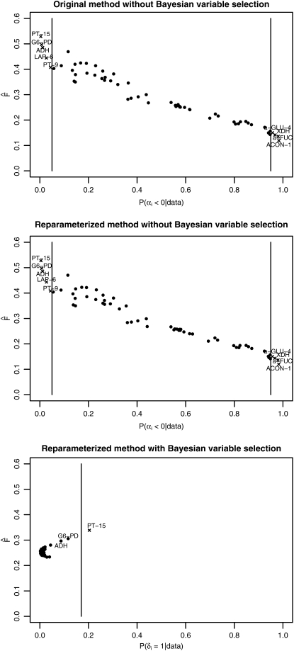
Beaumont and Balding (2004) identified 10 loci as being subject to selection. The newly implemented version detected 9 of these 10 loci. The locus EST-6 was not detected as being subject to balancing selection, but its Bayesian P-value is close to the critical value (see Table 7). All Bayesian P-values obtained are nearly identical to those obtained by Beaumont and Balding (2004), whereas the Fst-values show small differences (compare Table 7). Table 7 and Figure 2 show that the results of Beaumont and Balding (2004) could be reproduced, except for small deviations, indicating that the newly implemented version is correct.
TABLE 7.
Results for the Singh and Rhomberg (1987) data set
|
Fst
|
P-value
|
P(δi = 1 | data): | ||||||
|---|---|---|---|---|---|---|---|---|
| Locus | Article | Original | Reparameterized | Variable selection | Article | Original | Reparameterized | Variable selection |
| G6-PD | 0.47a | 0.50a | 0.50a | 0.31 | 0.00a | 0.01a | 0.01a | 0.12 |
| ADH | 0.45a | 0.49a | 0.49a | 0.30 | 0.01a | 0.01a | 0.01a | 0.09 |
| EST-6 | 0.18a | 0.15 | 0.15 | 0.24 | 0.95a | 0.94 | 0.94 | 0.01 |
| PT-9 | 0.43a | 0.41a | 0.41a | 0.27 | 0.05a | 0.04a | 0.04a | 0.02 |
| PT-15b | 0.52a | 0.53a | 0.53a | 0.34a | 0.00a | 0.00a | 0.00a | 0.20a |
| XDH | 0.13a | 0.14a | 0.14a | 0.23 | 0.98a | 0.98a | 0.98a | 0.03 |
| a-FUC | 0.14a | 0.14a | 0.14a | 0.24 | 0.97a | 0.97a | 0.97a | 0.02 |
| LAP-6 | 0.47a | 0.44a | 0.44a | 0.28 | 0.03a | 0.03a | 0.03a | 0.04 |
| ACON-1 | 0.15a | 0.12a | 0.12a | 0.23 | 0.99a | 0.98a | 0.98a | 0.04 |
| a-GLU-4 | 0.17a | 0.15a | 0.15a | 0.24 | 0.96a | 0.96a | 0.96a | 0.02 |
Estimated Fst-values for all methods, corresponding Bayesian P-values P(αi < 0 | data) for the original and the reparameterized algorithm, and corresponding posterior probabilities P(δi = 1 | data) for the reparameterized algorithm including Bayesian variable selection for loci detected being subject to selection by one of the methods are shown. Article, Beaumont and Balding (2004) results; Original, original algorithm; Reparameterized, reparameterized algorithm; Variable selection, reparameterized algorithm including Bayesian variable selection.
The locus is classified subject to selection by the corresponding method.
All methods classify the corresponding locus subject to selection.
Figure 2.—
Results from the analysis of the Singh and Rhomberg (1987) Drosophila melanogaster data set. Estimated Fst-values are plotted against empirical Bayesian P-values P(αi < 0 | data) for each locus in the case of the original and the reparameterized method without Bayesian variable selection. For the method including Bayesian variable selection the estimated Fst-values are plotted against the posterior probability P(δi = 1 | data). The vertical bars indicate the corresponding critical values used for identifying loci that might be subject to selection. Detected loci are marked with an “x.”
Comparison of the original and the reparameterized version:
The results of the reparameterized method are identical to those of the original model (see Table 7). This result was expected, because the reparameterization does not entail any changes to the algorithm. It is only a reformulation that increases efficiency by allowing us to sample directly from the full conditional distributions of αi and βj.
Efficiency:
The effective sample size ESS was calculated for all locus effects αi and then averaged; analogously the ESS was calculated for the population effects βj. Table 8 shows the results, with the last column presenting the relative efficiency of the reparameterized method over the original method, indicated by the relative effective sample size standardized for CPU run time. As expected, the reparameterization caused higher autocorrelations in the chain but led to an improvement in the standardized relative ESS. Considering this efficiency gain, the reparameterized version should be preferred. Therefore the original version was not considered further.
TABLE 8.
Performance comparison between the original and the reparameterized methods
| Original
|
Reparameterized
|
||||
|---|---|---|---|---|---|
| Coefficient | CPU (hr) | ESS | CPU (hr) | ESS | Relative ESS |
| α (I = 61) | 7.017 | 9680 | 3.595 | 6866 | 1.38 |
| β (J = 15) | 7.017 | 9045 | 3.595 | 6951 | 1.50 |
Analyzing the Singh and Rhomberg (1987) data set, the total CPU time was measured for both methods and the effective sample size (ESS) was calculated, as defined in Equation 3. The last column shows the relative effective sample size standardized for CPU run time, indicating the relative efficiency of the reparameterized method over the original method.
Results of the reparameterized method including Bayesian variable selection:
The results for the reparameterized method with variable selection are shown in Figure 2. Instead of the Bayesian P-values the posterior probabilities P(δi = 1 | data) were used to detect significant loci. The cutoff value is 0.17 as determined in the previous simulation studies.
Accuracy:
One of the 10 loci identified by Beaumont and Balding (2004) was detected as being subject to selection by the new method with Bayesian variable selection. No additional loci were considered significant. Beaumont and Balding (2004) showed by simulations that very few loci being subject to balancing selection were identified by their Bayesian hierarchical method, but if loci were classified as being subject to balancing selection, the identification was mostly correct. Beaumont and Balding (2004) detected 5 loci as being subject to balancing selection. However, none of these loci were inferred as being subject to balancing selection by the method with Bayesian variable selection.
Locus-by-population effects:
In accordance with Beaumont and Balding (2004) all methods found an extremely high γij value for the biallelic locus PT-26 in the West African sample and a significantly negative γij value for locus AO in the sample from Texas.
The highest posterior expectation E(αi + γij) was found for the triallelic locus G6-PD. In the sample from Texas, the allele that is the rarest in 13 of the other 14 populations is fixed. The reason could be a selective pressure at this locus that is absent in the other populations.
Analysis of tomato data:
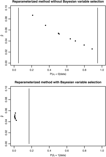
As a second example, we analyzed the sequence data set from S. chilense. This data set includes large DNA regions, and nearly every haplotype represents a new allele; e.g., the number of unique haplotypes is high. Figure 3 shows that there were no locus effects classified as significant. All Fst-values are very close to zero, indicating that there are no signatures of directional selection in the data. However, as all Fst-values are small, it seems probable that the haplotype counts contained too little information about genetic differentiation.
Figure 3.—
Results from the analysis of the S. chilense data set. Estimated Fst-values are plotted against empirical Bayesian P-values P(αi < 0 | data) for each locus in the case of the reparameterized method without Bayesian variable selection. For the method including Bayesian variable selection the estimated Fst-values are plotted against the posterior probability P(δi = 1 | data). The vertical bars indicate the corresponding critical values used for identifying loci that might be subject to selection.
Accuracy:
This tomato data set is a typical extreme data set in the sense of Hudson et al. (1992a). Arunyawat et al. (2007) estimated parameters of genetic differentiation with the program DnaSP version 4.0 (Rozas et al. 2003), which, in addition to haplotype-based methods, used nucleotide-based methods. The nucleotide-based statistics by Hudson et al. (1992b) obtained clearly higher values than the haplotype-based ones. For example, for locus CT208, an Fst-value of 0.340 was obtained (compare Arunyawat et al. 2007, Table 4). This value indicates positive directional selection, whereas the value obtained by the methods developed here hints toward balancing selection as a more likely alternative. The haplotype-based statistics by Nei (1973) used in DnaSP also yielded smaller values than the nucleotide-based statistics.
DISCUSSION
Many previous studies have used Bayesian P-values to identify loci subject to selection (e.g., Beaumont and Nichols 1996; Beaumont and Balding 2004). Here, we presented two extensions of an algorithm developed by Beaumont and Balding (2004) to automatically select nonneutrally behaving loci by introducing Bayesian variable selection. First, we reparameterized the model framework and showed that this increases the efficiency. Then we introduced a new Bayesian auxiliary variable to decide whether a locus is subject to selection.
We applied the reparameterized method with and without Bayesian variable selection to a fruit fly allozyme data set, to a wild tomato sequence data set, and to simulated data sets from a Wright–Fisher model with migration. ROC analyses showed that the method with variable selection performs significantly better than the method without variable selection.
The new approach described here leads to important advantages of interpretation, since it is now possible to evaluate the predictions by scoring rules. Such an analysis is not possible using the Beaumont and Balding (2004) approach, as there are no probabilities available for the hypothesis that a locus is neutral and hence has a zero locus effect. Scoring rules measure the quality of predictions by assigning a numerical score. An often-used scoring rule for binary data is the Brier score that measures the disagreement between the observed outcome and the prediction probability of that outcome—the average squared error difference. The Brier score is a measure of overall accuracy and can be decomposed into aspects of calibration and discrimination (Spiegelhalter 1986). A perfect forecaster would have a Brier score of 0 and a perfect misforecaster a Brier score of 1. Although the numerical value has no direct meaning, some weak standards for comparison are available. One reference value is obtained by noting that a prediction probability of 0.5 for each locus results in a Brier score of 0.25. Another reference value is the outcome index variance, which is the value of the Brier score if all prediction probabilities were equal to the prevalence (Schmid and Griffith 2005). With a prevalence of 10% the outcome index variance in our simulations is 0.09, which can be used as a natural upper bound. For the method including Bayesian variable selection we got Brier scores <0.05. We also calculated a mean discrimination, defined as the difference between the average predicted probabilities in the selected and the neutral group, between 51 and 59%. The discrepancy between the mean forecast and the observed fraction of selection events is between 0.02 and 0.03. This low bias was expected as we classified a locus subject to selection with a prior expectation of 10%, which is equal to the prevalence in the simulations. However, we found that even classifying a locus subject to selection with an expected prior probability of 50% by using a uniform prior distribution does not increase this bias.
A disadvantage of the presented methods is that they are based on haplotype statistics. Using sequence data sets, every distinct haplotype is treated as a new allele, independent of the number of differing nucleotides. Therefore, when applying the methods to data sets where many haplotypes are unique, the calculated haplotype frequencies may not reflect the amount of information on genetic differentiation that is included in the sequence data. As in the wild tomato example, all methods would classify the loci as neutral with Fst-values close to zero. Hudson et al. (1992a) showed that models based on haplotype statistics are very powerful for data sets having low mutation rates or large sample sizes, as was the case in the Singh and Rhomberg (1987) data set. However, for data sets with high mutation rates or small sample sizes, as in the wild tomato example, the sequence-based statistics are expected to be more powerful. Therefore, the integration of nucleotide-based statistics will be a clear improvement. Ideally, the appropriate method would be chosen according to the data set under study.
Acknowledgments
We are grateful to Mark Beaumont for helpful comments and thank the associate editor and two anonymous reviewers for valuable comments on a previous version of this article. A.R. and L.H. acknowledge support from the Swiss Science Foundation. W.S. thanks the Deutsche Forschungsgemeinschaft (project STE 325/5) for support.
APPENDIX A: SIMULATION STUDY DESIGN
We used a Wright–Fisher model with migration to generate simulated data sets. It is nearly the same simulation model as that used in Beaumont and Balding (2004), but without the possibility for mutations.
The simulation model for a particular locus i and a particular population j is as follows:
Decide whether locus i for population j is neutral, subject to directional selection, or subject to balancing selection.
Determine randomly the attribute (blue, b; red, r; or neutral, n) for population j at locus i with pb,j = 0.4, pr,j = 0.4, and pn,j = 0.2 as proposed by Beaumont and Balding (2004).
- Sample the next generation
 having population size N:
Determine the observed allele frequencies
 .
.- Replace a binomially distributed number of chromosomes in population j by immigrants chosen at random from all other populations. Each immigrant replaces a randomly chosen resident chromosome as follows:
- Calculate the immigration rate
 whereby F is either sampled from a beta distribution with parameters 0.25 and 2.25 as given in Beaumont and Balding (2004), so that the immigration rate is variable over the populations, or set to a fixed value (e.g., 0.2).
 - Determine the number of immigrants
 into population j.
 - Determine the chromosomes in population j that should be replaced:

- Determine where the immigrants come from,
where

- Determine the chromosome type of the immigrant chromosomes,
with
 .
. - Replace the selected resident chromosomes with the immigrant chromosomes.
-
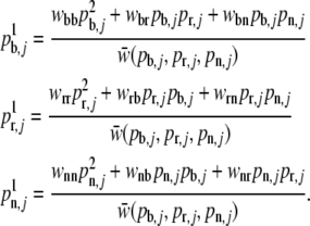
Determine the relative fitness w assuming a diploid selection model with alleles “blue (b),” “red (r),” and “neutral (n).” The relative fitness depends on the type of selection:
- For loci subject to directional selection, the relative fitness in a blue population is 1 + s for blue homozygotes,1+s/2 for blue heterozygotes, and 1 for all other genotypes. The same selection effects are assumed for red alleles in red populations. In neutral populations all genotypes have a relative fitness of 1.
- For loci subject to balancing selection in either red or blue populations the relative fitness of blue–red heterozygotes is 1 + s and for all other genotypes 1. In neutral populations all genotypes have fitness 1.
- For neutral loci all genotypes have fitness 1.
Calculate the mean fitness of population j assuming Hardy–Weinberg equilibrium and calculate the allele proportions for the next generation with
and
Set
 and go to step 3.
APPENDIX B: ROC ANALYSIS
This section is devoted to the evaluation of the classification quality of the different models. We assume to have nD test results for loci subject to selection and  test results for neutral loci:
 |
It is assumed that {YD,s, s = 1, …, nD} are identically distributed with survivor function SD(y) = P(YD,s ≥ y), and similarly  are such that
  .
.
Before we calculated empirical AUC values for all simulated data sets, we deleted ties in the test results by adding random noise. We did the calculations separately for the method without Bayesian variable selection and the method with Bayesian variable selection. In these calculations we did not distinguish between loci subject to balancing and positive directional selection.
The asymptotic variance for the AUC estimates was estimated by
where AUC, Q1, and Q2 were calculated as described in Hanley and McNeil (1982).
To compare the ROC curves for the method with variable selection and the method without variable selection we used the difference in empirical AUC estimates. As the ROC curves for both methods are derived from the same data sets, we have a paired study design, so that the variance of  is given by
which is estimated with
 |
(A1) |
where A is the index for the method with variable selection and B the index for the method without variable selection. In Equation A1 empirical placement values are used for the calculation of the empirical variance. A placement value for a test result y in the neutral distribution, for example, is defined as
 |
where the distribution of  is considered as the reference distribution (Pepe 2003).
References
- Arunyawat, U., W. Stephan and T. Städler, 2007. Using multilocus sequence data to assess population structure, natural selection and linkage disequilibrium in wild tomatoes. Mol. Biol. Evol. 24 2310–2322. [DOI] [PubMed] [Google Scholar]
- Balding, D. J., 2003. Likelihood-based inference for genetic correlation coefficients. Theor. Popul. Biol. 63 221–230. [DOI] [PubMed] [Google Scholar]
- Balding, D. J., and R. A. Nichols, 1995. A method for quantifying differentiation between populations at multi-allelic loci and its implications for investigating identity and paternity. Genetica 96 3–12. [DOI] [PubMed] [Google Scholar]
- Beaumont, M. A., and D. J. Balding, 2004. Identifying adaptive genetic divergence among populations from genome scans. Mol. Ecol. 13 969–980. [DOI] [PubMed] [Google Scholar]
- Beaumont, M. A., and R. A. Nichols, 1996. Evaluating loci for use in the genetic analysis of population structure. Proc. R. Soc. Lond. Ser. B 263 1619–1626. [Google Scholar]
- Bernardo, J. M., and A. F. M. Smith, 1994. Bayesian Theory. John Wiley & Sons, Chichester, UK.
- Besag, J., P. Green, D. Higdon and K. Mengersen, 1995. Bayesian computation and stochastic systems. Stat. Sci. 10 3–41. [Google Scholar]
- Bonin, A., P. Taberlet, C. Miaud and F. Pompanon, 2006. Explorative genome scan to detect candidate loci for adaption along a gradient of altitude in the common frog (Rana temporaria). Mol. Biol. Evol. 23 773–783. [DOI] [PubMed] [Google Scholar]
- Dellaportas, P., J. J. Forster and I. Ntzoufras, 2002. On Bayesian model and variable selection using MCMC. Stat. Comput. 12 27–36. [Google Scholar]
- Gelman, A., G. O. Roberts and W. R. Gilks, 1996. Efficient Metropolis jumping rules, pp. 599–607 in Bayesian Statistics, Vol. 5, edited by J. M. Bernardo, J. O. Berger, A. P. Dawid and A. F. M. Smith. Oxford University Press, London/New York/Oxford.
- Geyer, C. J., 1992. Practical Markov chain Monte Carlo. Stat. Sci. 7 473–511. [Google Scholar]
- Gilks, W. R., S. Richardson and D. J. Spiegelhalter, 1996. Markov Chain Monte Carlo in Practice. Chapman & Hall, London.
- Glinka, S., L. Ometto, S. Mousset, W. Stephan and D. De Lorenzo, 2003. Demography and natural selection have shaped genetic variation in Drosophila melanogaster: a multi-locus approach. Genetics 165 1269–1278. [DOI] [PMC free article] [PubMed] [Google Scholar]
- Hanley, J. A., and B. J. McNeil, 1982. The meaning and use of the area under the receiver operating characteristic (ROC) curve. Radiology 143 29–36. [DOI] [PubMed] [Google Scholar]
- Holmes, C., and L. Held, 2006. Bayesian auxiliary variable models for binary and multinomial regression. Bayesian Anal. 1 145–168. [Google Scholar]
- Hudson, R. R., D. D. Boos and N. L. Kaplan, 1992. a A statistical test for detecting geographic subdivision. Mol. Biol. Evol. 9 138–151. [DOI] [PubMed] [Google Scholar]
- Hudson, R. R., M. Slatkin and W. P. Maddison, 1992. b Estimation of levels of gene flow from DNA sequence data. Genetics 132 583–589. [DOI] [PMC free article] [PubMed] [Google Scholar]
- Kass, R. E., B. P. Carlin, A. Gelman and R. M. Neal, 1998. Markov chain Monte Carlo in practice: a roundtable discussion. Am. Stat. 52 93–100. [Google Scholar]
- Li, H., and W. Stephan, 2006. Inferring the demographic history and rate of adaptive substitution in Drosophila. PLoS Genet. 2 e166. [DOI] [PMC free article] [PubMed] [Google Scholar]
- Mealor, B. A., and A. L. Hild, 2006. Potential selection in native grass populations by exotic invasion. Mol. Ecol. 15 2291–2300. [DOI] [PubMed] [Google Scholar]
- Nei, M., 1973. Analysis of gene diversity in subdivided populations. Proc. Natl. Acad. Sci. USA 70 3321–3323. [DOI] [PMC free article] [PubMed] [Google Scholar]
- Pepe, M. S., 2003. The Statistical Evaluation of Medical Tests for Classification and Prediction. Oxford University Press, Oxford.
- Ronald, J., and J. M. Akey, 2005. Genome-wide scans for loci under selection in humans. Hum. Genomics 2 113–125. [DOI] [PMC free article] [PubMed] [Google Scholar]
- Rozas, J., J. C. Sánchez-DelBarrio, X. Messeguer and R. Rozas, 2003. DnaSP, DNA polymorphism analyses by the coalescent and other methods. Bioinformatics 19 2496–2497. [DOI] [PubMed] [Google Scholar]
- Schmid, C. H., and J. L. Griffith, 2005. Multivariate classification rules: calibration and discrimination, pp. 3491–3497 in Encyclopedia of Biostatistics, Vol. 5, Ed. 2, edited by P. Armitage and T. Colton. Wiley, Chichester, UK.
- Singh, R. S., and L. R. Rhomberg, 1987. A comprehensive study of genic variation in natural populations of Drosophila melanogaster. II. Estimates of heterozygosity and patterns of geographic differentiation. Genetics 117 255–271. [DOI] [PMC free article] [PubMed] [Google Scholar]
- Spiegelhalter, D. J., 1986. Probabilistic prediction in patient management and clinical trials. Stat. Med. 5 421–433. [DOI] [PubMed] [Google Scholar]
- Vasemägi, A., J. Nilsson and C. R. Primmer, 2005. Expressed sequence tag-linked microsatellites as a source of gene-associated polymorphisms for detecting signatures of divergent selection in Atlantic salmon (Salmo salar L.). Mol. Biol. Evol. 22 1067–1076. [DOI] [PubMed] [Google Scholar]
- Wright, S., 1943. Isolation by distance. Genetics 28 114–138. [DOI] [PMC free article] [PubMed] [Google Scholar]


